Advanced data processing

Pairwise distribution

Once a proper Guinier analysis is achieved and there is no indication of molecular aggregation or repulsion, the calculation of the pairwise distribution function $P(r)$ , the inverse Fourier transform (IFT) of $I(q)$ vs $q$ , is the next step in the analysis of the SAXS data. Several softwares have been developped, including GNOM and the Bayesian IFT approaches.

The $P(r)$ function describes the distribution of all electron-pair distances within the sample. This function will be characteristic of the shape of the sample. An illustration taken from Mertens and Svergun (2010) is given below.

I(q) vs q, P(r) function

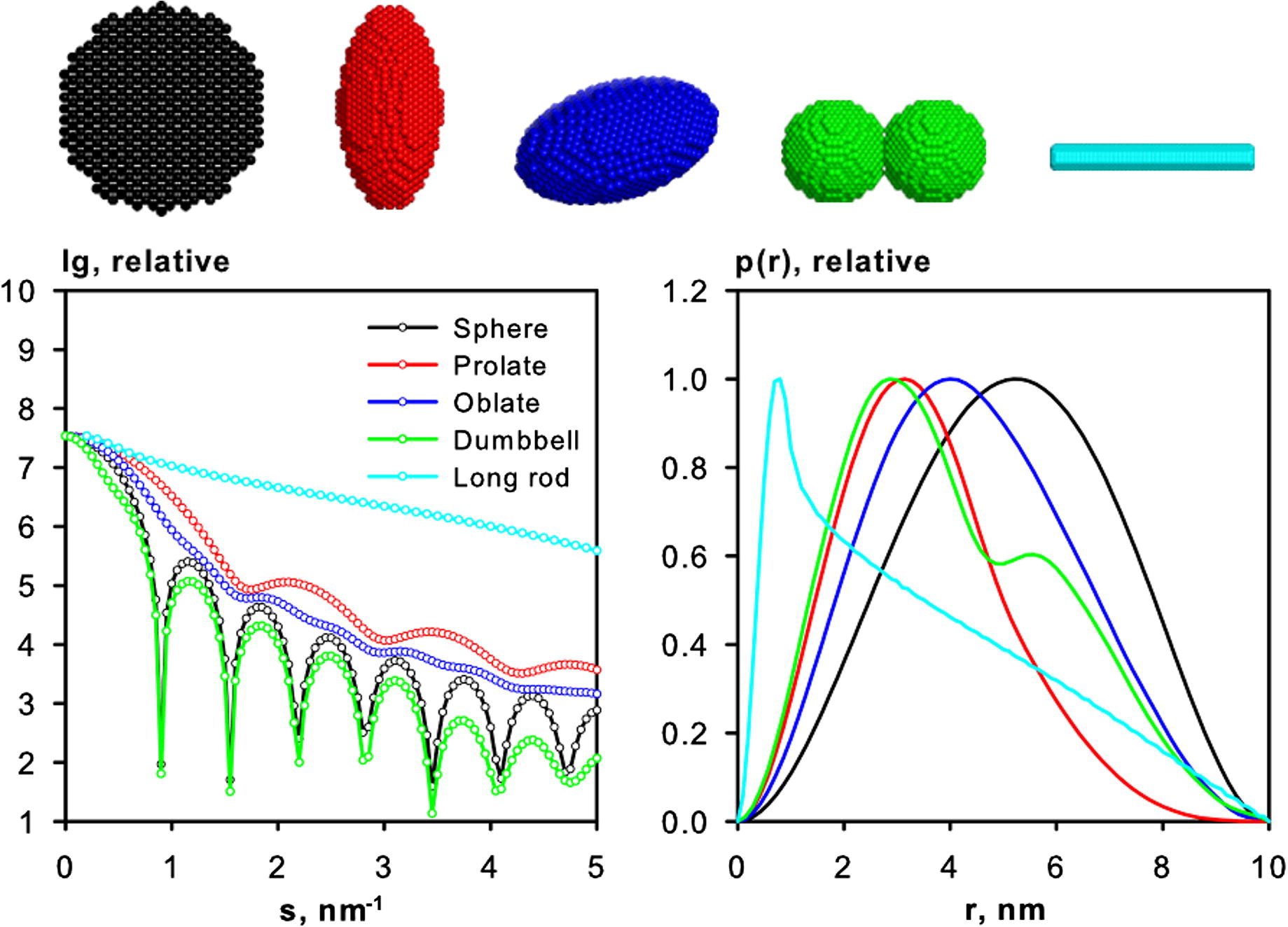
Source: Mertens and Svergun (2010)

From the $P(r)$ function, both $R_g$ and $D_{max}$ can be determined using the full range of $q$ experimental data. Here, $D_{max}$ represents the maximum diameter in the sample particle. Globular samples will have a $P(r)$ function with a single peak (black curve), and the more spherical the particle, the more symmetric will the $P(r)$ function be. Alternatively, irregular, or elongated particles, will have a longer "tail" at large $r$ (see the cyan curve above) and may exhibit multiple peaks in the function (see the green curve above).

GNOM

The most common such method is implemented in the GNOM program from the ATSAS package (Franck et al. 2017). In RAW, using the buffer-substracted data (S_A_<experiment_number><sample_name> file), the software can be accessed with a right-click on the filename and choosing the option IFT (GNOM). A new window will open and a $P(r)$ function will be generated (top plot), along with the corresponding fit to the experimental data (bottom plot).

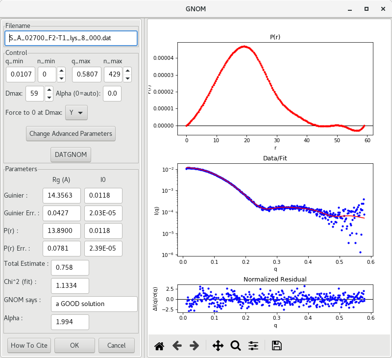
Initial approximations of $I(0)$ , $R_g$ and $D_{max}$ values are reported, along with their uncertainties. The previously obtained Guinier approximation results are reported also so one can compare the results of the different approaches. They generally should agree well.

An assessment of the quality of the function is nonetheless important. GNOM will report a Total Estimate (TE), which varies from 0 (no agreement between experimental data and the fit) to 1 (perfect match). A quick way to verify is also to read the GNOM says output. Depending on the total estimate, GNOM will say Excellent (TE $≥$ 0.9), Good (0.9 $>$ TE $≥$ 0.75), Reasonable (0.75 $>$ TE $≥$ 0.5) or Suspicious (TE $<$ 0.5).

It is very important, as you will see below, when using GNOM to look for suspicious results. For example, the $P(r)$ function should reach zero "smoothly" at $D_{max}$ . By default, the option Force to 0 at Dmax is set to Y. One way to verify this is to set Force to 0 at Dmax to N and observe the shape of the curve at $D_{max}$ . For high quality data, the function will get to 0 whether it is forced or not.

Any result being suspicious should be analyzed carefully and is likely not of good quality to move forward in the processing of the data.

It is also possible to change the values of q_min, q_max in order to exclude erronous data at low or high $q$ , or even adjust the value of $D_{max}$ in order to smooth out the curve towards 0 at high $q$ .

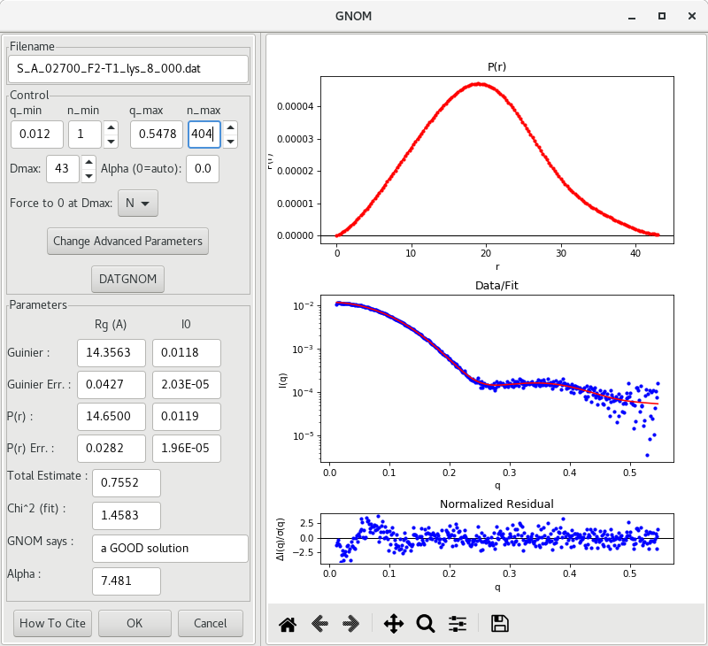
As you can see in the example in this tutorial (above), we get a more realistic $P(r)$ function following small adjustments while still keeping a good Total Estimate (above 0.75). Also, $R_g$ and $I(0)$ determined by the $P(r)$ function agree well with the Guinier estimates.

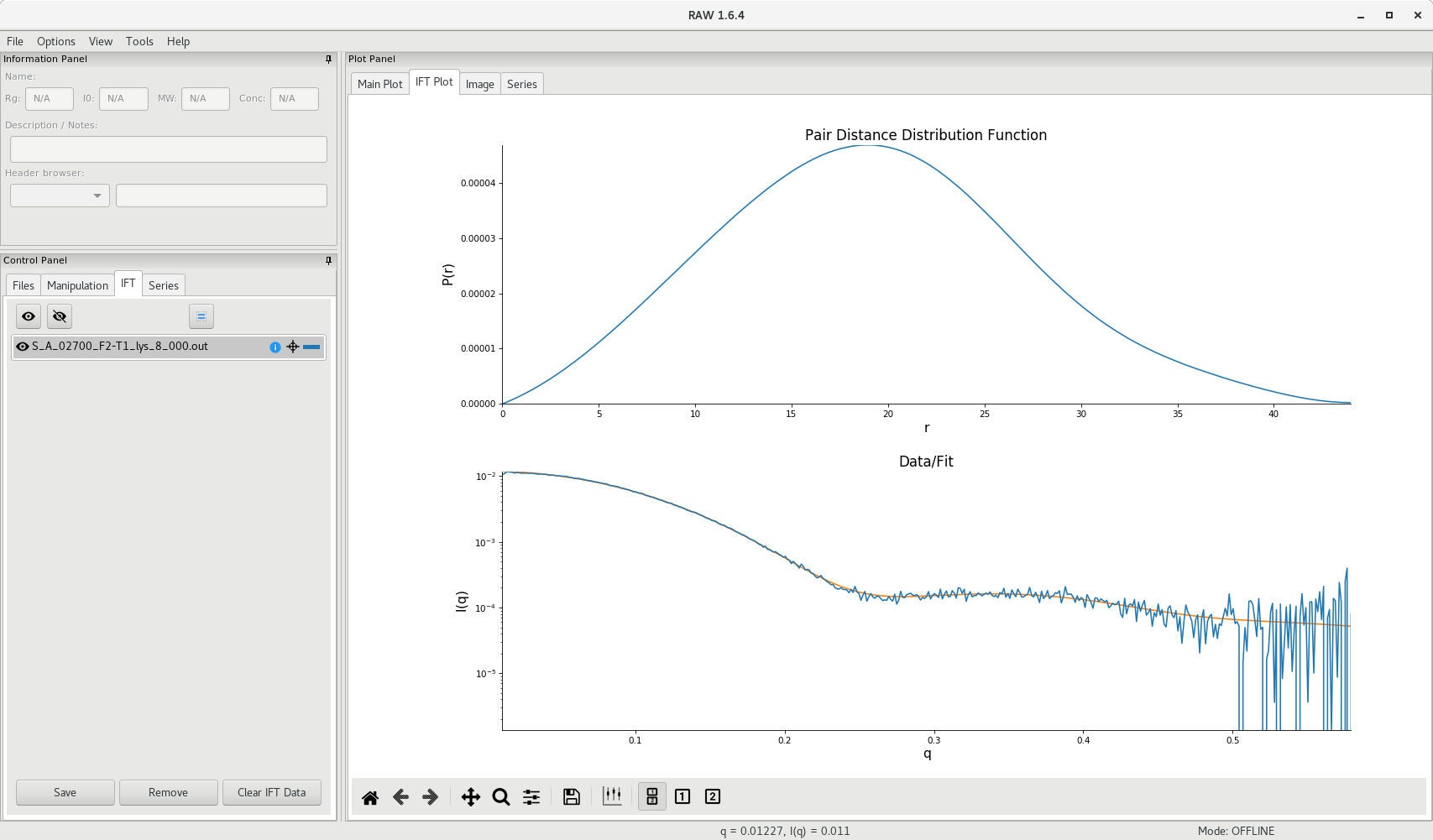
Do not forget to save your data (the .out file) in the processed_data subdirectory:

<project_name>/processed_data/GNOM/S_A_<experiment_number><sample_name>.out

This file will be used later as input for DAMMIF for dummy atom modelling, or for DENSS for electron density modelling.

BIFT

A Bayesian approach for calculating the pairwise distribution function $P(r)$ , first proposed by Hansen (2000), is another way of calculating the pairwise distribution function $P(r)$ . In RAW, using the buffer-substracted data (S_A_<experiment_number><sample_name>.dat file), the software can be accessed with a right-click on the filename and choosing the option IFT (BIFT). A new window will open and a $P(r)$ function will be generated (top plot), along with the corresponding fit to the experimental data (bottom plot).

Similar to the output of GNOM, values of $I(0)$ , $R_g$ and $D_{max}$ are reported, along with their uncertainties. This method has the advantage of having only one solution, and parameters cannot be adjusted. The previously obtained Guinier approximation results are reported also so one can compare the results of the different approaches. They generally should agree well.

One caveat of the BIFT method is that the output file is not compatible with DAMMIF for dummy atom modelling, but can be used for DENSS for electron density modelling.